
Bunny graph diffusion
We scale the small graph walk's edge-local PSWAP rule up to diffusion on the Stanford bunny's mesh connectivity. Torx supplies the sampled full-graph result, and NumPy supplies the ordered-sweep mean plus the exact graph-diffusion reference, which is how we tell sampling noise apart from the error of the ordered sweep itself.
The Stanford bunny is usually presented as a surface, but its mesh also defines a graph: vertices become nodes and triangle sides become edges. How can the edge-local PSWAP rule from notebook 02 reproduce diffusion on this graph when the same rule must be applied across a few hundred vertices?
We begin with a single excitation at one ear vertex. Each unweighted mesh edge contributes one PSWAP gate, and $x_i(t)$ denotes the probability that the excitation occupies vertex $i$ after averaging repeated one-hot runs. Every run therefore places the excitation on exactly one vertex, while the average over runs gives a probability field on the graph.
This construction follows from the combinatorial graph Laplacian $L = D - A$, which splits into one symmetric two-node term per edge. A layer of ordered PSWAP gates approximates the simultaneous graph evolution, and repeating the layer propagates probability through the connectivity graph.
A sampled field alone does not tell us whether a discrepancy comes from finite sampling or from the ordered approximation. We therefore compare the full Torx result with two NumPy references. The deterministic ordered-sweep mean applies exactly the same updates without sampling, which isolates sampling error. The exact graph-diffusion solution then exposes the error introduced by the finite ordered sweep itself. Finally, we repeat the parity comparison on a closed 32-vertex patch, where the result can be inspected vertex by vertex.
Throughout the notebook, diffusion refers only to the unweighted connectivity graph. It is not a model of physical heat flow over the surface: edge lengths, triangle angles, vertex areas, and a mesh mass matrix do not enter the construction.
Setup
First we put the local helpers directory on the import path, then import Torx and NumPy.
from pathlib import Path
import sys

ROOT = Path.cwd()
if not (ROOT / "helpers").exists() and (ROOT.parent / "helpers").exists():
    ROOT = ROOT.parent
HELPER_DIR = ROOT / "helpers"
# Put shared notebook helpers on the import path.
sys.path.insert(0, str(HELPER_DIR))
from collections import deque

import numpy as np

from torx.psc import DiscretePCircuit, PSWAP
Several actors contribute to the numbers below, so we say up front which one produces what.
What runs where?
- Torx executes the repeated
PSWAPcircuits and returns sampled occupancies. - Notebook code exposes the full circuit and reports the three error numbers: sampling error, splitting bias (what the ordered per-edge sweep gets wrong on its own), and total error.
examples/helpers/_graph_diffusion.pyprovides NumPy references and Torx sampling wrappers, whileexamples/helpers/_stanford_bunny.pyloads, decimates, keeps the largest connected component, and plots the mesh.- The offline mesh is
examples/assets/stanford_bunny/bun_zipper_res3.ply.
from _notebook_paths import figure_dir
from _notebook_style import apply_notebook_style, make_savefig
from _graph_diffusion import (
    _edge_swap_probability as shared_edge_swap_probability,
    build_graph_generator,
    ordered_pswap_product_formula_mean,
    reference_heat_flow,
    sample_pswap_product_formula,
    sample_pswap_product_formula_multiseed,
)
from _stanford_bunny import (
    decimate_mesh,
    largest_connected_mesh,
    load_ascii_ply,
    mesh_edges,
    save_torx_reference_figure,
    visible_source_vertex,
)
We keep the plotting style and the figure output path in the plotting helpers and import mesh preprocessing from the mesh helper above, which leaves the cells below free to talk about the graph itself.
import _plots_sampling as P_samp
import _plots_schematics as P_sch

apply_notebook_style()
FIGURE_DIR = figure_dir(ROOT)
savefig = make_savefig(FIGURE_DIR)
MESH_PATH = ROOT / "assets" / "stanford_bunny" / "bun_zipper_res3.ply"
assert MESH_PATH.exists(), MESH_PATH
Graph connectivity, the Laplacian, and one swap per edge
Before applying a circuit to a graph with a few hundred vertices, we establish why one two-site gate per edge can represent a step of graph diffusion.
A triangle mesh induces a graph $G = (V, E)$: each vertex is a pbit, and each triangle side contributes an unweighted edge. Let $A$ be the adjacency matrix and $D$ the degree matrix. Their difference, the combinatorial graph Laplacian $L = D - A$, compares the value at each vertex with the values at its neighbors. Graph diffusion is then defined by
$$ \dot x = -Lx, \qquad x(t) = e^{-Lt}x(0). $$
Under this equation, probability moves only between adjacent vertices. This is the master equation from notebook 02, with generator $Q=-L$.
To connect this simultaneous evolution to edge-local gates, we use the decomposition $L=\sum_{(i,j)\in E}L_{ij}$, in which each $L_{ij}$ is a symmetric two-node block. Lie-Trotter splitting rewrites the exact propagator as the limit of ordered products over these blocks:
$$ x(t) = \lim_{N\to\infty}\Bigl(\underbrace{\textstyle\prod_{(i,j)\in E}e^{\Delta t Q_{ij}}}_{\vphantom{\big|}\text{ordered per-edge sweep}}\Bigr)^N x(0), \qquad \Delta t=t/N. $$
For finite $N$, Torx evaluates each product as a sequential sweep over the edge list. On this unit-rate graph, each factor $e^{\Delta t Q_{ij}}$ is one PSWAP with $p=\tfrac12(1-e^{-2\Delta t})$. Overlapping factors share a vertex and do not commute, so the finite ordered product differs from $e^{-Lt}$. We call this residual difference the splitting bias and measure it below.
Torx constructs only the per-edge factors and never forms the dense propagator $e^{-Lt}$. NumPy consequently provides both references used in the comparison: the exact eigensolution and the deterministic mean of the same ordered sweep.
Diffusion on the bunny connectivity graph
We now construct the graph and define what each of the two diffusion figures is intended to compare.
All probability begins at one ear vertex and then spreads along graph edges. We load the bun_zipper_res3 reconstruction from the Stanford bunny dataset, retain its largest connected component, and coarsen it with decimate_mesh from examples/helpers/_stanford_bunny.py. The decimator snaps vertices to a uniform 3-D grid, replaces occupied cells with centroids, remaps faces, and drops collapsed triangles. This preprocessing produces the 450-vertex, 1,352-edge graph used below.
Torx samples the full graph only at $t=1.5$. Sampling $t=10$ or $t=40$ by the same construction would require many more repetitions of every gate in the layer, each evaluated over its own batch of samples. The $t=10$ and $t=40$ panels are therefore NumPy exact references, not Torx results.
The two figures answer different questions and use different color conventions. The same-time comparison places the Torx and NumPy fields on a shared absolute scale, so the same color denotes the same probability in both panels. The time progression instead normalizes each panel by its own peak. This keeps the later, flatter fields visible, but it no longer encodes the decrease in absolute magnitude; each panel title therefore reports its unnormalized peak.
raw_vertices, raw_faces = load_ascii_ply(MESH_PATH)
full_vertices, full_faces = largest_connected_mesh(raw_vertices, raw_faces)

# Grid-snap the mesh to define the smaller connectivity graph used below.
TARGET_VERTICES = 400
vertices, faces = decimate_mesh(full_vertices, full_faces, TARGET_VERTICES)
vertices, faces = largest_connected_mesh(vertices, faces)
edges = mesh_edges(faces)
source = visible_source_vertex(vertices)
assert len(full_vertices) == 1_887  # full largest connected component
assert 250 <= len(vertices) <= 600  # coarsened, still bunny-shaped
assert len(edges) >= len(vertices)  # connected graph
# TORX_STEPS is tuned to this realized coarse graph size.
# Changing the mesh or target size requires retuning the step count.
print(f"full mesh:    {len(full_vertices)} vertices")
print(f"coarse mesh:  {len(vertices)} vertices, {len(faces)} faces, {len(edges)} edges")
print(f"source:       vertex {int(source)}")
full mesh:    1887 vertices
coarse mesh:  450 vertices, 932 faces, 1352 edges
source:       vertex 239
# Build the continuous-time generator for the unweighted connectivity graph.
generator = build_graph_generator(len(vertices), edges, rate=1.0)
initial = np.zeros(len(vertices))
initial[int(source)] = 1.0

TORX_TIME, TORX_STEPS = 1.5, 11
TORX_SAMPLES_PER_SEED = 8_000
TORX_SEEDS = (17, 29, 43, 59)
reference_times = [1.5, 10.0, 40.0]
We build the circuit here in the notebook rather than inside a helper, so every ingredient stays visible: one structural PSWAP per mesh edge, one common logit for the unit-rate slice probability, and reps=TORX_STEPS for the repeated layer. The shared sampler compiles and executes this same circuit for each seed.
p_edge = shared_edge_swap_probability(1.0, TORX_TIME, TORX_STEPS)
full_pswap_layer = [PSWAP([int(i), int(j)]) for i, j in edges]
full_torx_circuit = DiscretePCircuit(full_pswap_layer, reps=TORX_STEPS)
gate_applications = len(full_torx_circuit.gates) * full_torx_circuit.reps

print(
    f"{len(full_torx_circuit.gates):,} Torx PSWAP gates x "
    f"{full_torx_circuit.reps} reps = {gate_applications:,} gate applications"
)
print(f"per-edge swap probability: {p_edge:.4f}")
1,352 Torx PSWAP gates x 11 reps = 14,872 gate applications
per-edge swap probability: 0.1193
torx_fields = sample_pswap_product_formula_multiseed(
    initial,
    edges,
    reps=TORX_STEPS,
    swap_probability=p_edge,
    num_samples=TORX_SAMPLES_PER_SEED,
    seeds=TORX_SEEDS,
)
torx_field = torx_fields.mean(axis=0)
# NumPy references: exact graph diffusion and the deterministic mean of the
# same finite ordered edge sweep that Torx samples.
exact_fields = [
    reference_heat_flow(initial, generator, t) for t in reference_times
]
ordered_mean = ordered_pswap_product_formula_mean(
    initial,
    edges,
    reps=TORX_STEPS,
    swap_probability=p_edge,
)


def vertex_fraction_above_relative_peak(field):
    """Fraction of vertices above 15% of this field's peak."""
    return float(np.mean(field > 0.15 * field.max()))


uniform = np.full(len(vertices), 1.0 / len(vertices))
uniform_l2 = [float(np.linalg.norm(field - uniform)) for field in exact_fields]
# Three distances, three questions, as described in the markdown cell below:
# sampling error is Torx against the same ordered sweep computed exactly,
# splitting bias is that ordered sweep against exact graph diffusion, and total
# error is Torx against exact. They measure different things and need not add
# exactly.
sampling_l2 = float(np.linalg.norm(torx_field - ordered_mean))
splitting_bias_l2 = float(
    np.linalg.norm(ordered_mean - exact_fields[0])
)
total_l2 = float(np.linalg.norm(torx_field - exact_fields[0]))
per_seed_total_l2 = np.linalg.norm(torx_fields - exact_fields[0], axis=1)

np.testing.assert_allclose(torx_fields.sum(axis=1), 1.0, atol=8e-3)
assert exact_fields[0].max() > exact_fields[-1].max()
assert vertex_fraction_above_relative_peak(
    exact_fields[-1]
) > vertex_fraction_above_relative_peak(exact_fields[0])
assert uniform_l2[-1] < uniform_l2[0]
print("field                 peak     vertices > 15% of own peak")
print(
    f"Torx mean t={TORX_TIME:<4g}    {torx_field.max():.3f}        "
    f"{vertex_fraction_above_relative_peak(torx_field):.0%}"
)
for t, field in zip(reference_times, exact_fields, strict=True):
    print(
        f"NumPy exact t={t:<4g}  {field.max():.3f}        "
        f"{vertex_fraction_above_relative_peak(field):.0%}"
    )

print(f"\nTorx mean vs ordered-sweep mean, sampling L2: {sampling_l2:.4f}")
print(f"ordered-sweep mean vs NumPy exact, splitting bias L2: {splitting_bias_l2:.4f}")
print(f"Torx mean vs NumPy exact, total L2: {total_l2:.4f}")
print(
    f"per-seed total L2, mean +/- SD over {len(TORX_SEEDS)} seeds: "
    f"{per_seed_total_l2.mean():.4f} +/- {per_seed_total_l2.std(ddof=1):.4f}"
)
print(f"NumPy exact t=40 distance from uniform, L2: {uniform_l2[-1]:.4f}")
field                 peak     vertices > 15% of own peak
Torx mean t=1.5     0.040        9%
NumPy exact t=1.5   0.037        9%
NumPy exact t=10    0.017        27%
NumPy exact t=40    0.004        100%

Torx mean vs ordered-sweep mean, sampling L2: 0.0051
ordered-sweep mean vs NumPy exact, splitting bias L2: 0.0159
Torx mean vs NumPy exact, total L2: 0.0154
per-seed total L2, mean +/- SD over 4 seeds: 0.0176 +/- 0.0026
NumPy exact t=40 distance from uniform, L2: 0.0172
save_torx_reference_figure(
    vertices,
    faces,
    panels=[
        (
            f"Torx mean, {len(TORX_SEEDS)} seeds x {TORX_SAMPLES_PER_SEED // 1000}k\n"
            f"t={TORX_TIME:g}, total L2={total_l2:.3f}",
            torx_field,
        ),
        (f"NumPy exact reference\nt={reference_times[0]:g}", exact_fields[0]),
    ],
    output_stem=FIGURE_DIR / "03_bunny_graph_heat_flow",
    ncols=2,
    normalization="shared",
)
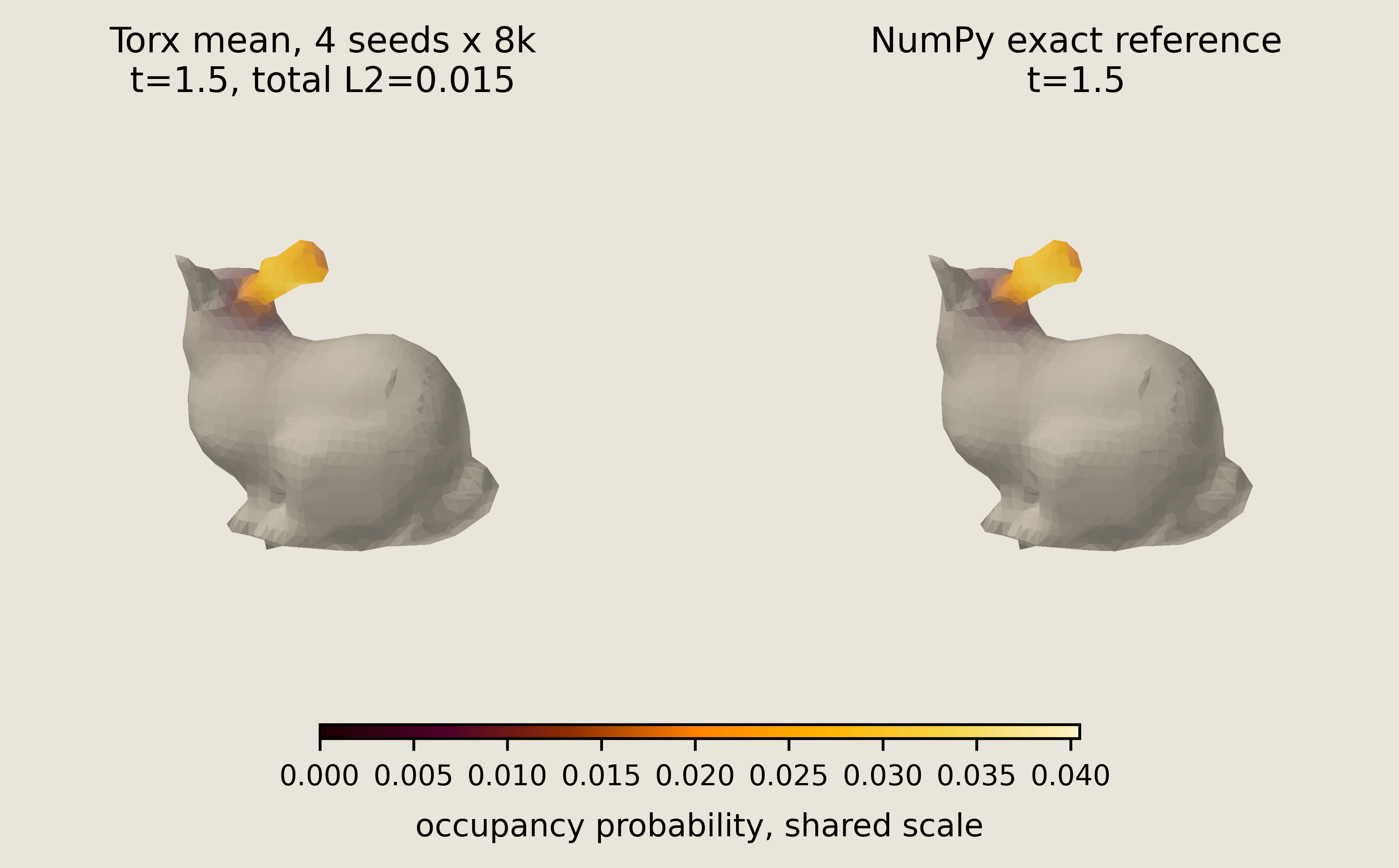
The first figure compares the Torx multi-seed mean with the NumPy exact field at the same $t=1.5$. Because the panels share an absolute color scale, equal colors represent equal probabilities. Both fields remain concentrated near the source: their peaks are 0.040 and 0.037, and 9% of vertices lie above 15% of each field's own peak.
The three distances separate the sources of the remaining difference. The sampling L2 of 0.0051 compares the Torx mean with the deterministic NumPy mean of the identical ordered sweep—same edge order, repetition count, and swap probability—so it measures sampling error alone. The splitting bias L2 of 0.0159 compares that ordered-sweep mean with exact graph diffusion, isolating the finite-$N$ approximation. Finally, the total L2 of 0.0154 compares Torx directly with the exact field and therefore includes both effects. These errors are vector differences rather than independent scalar contributions, so partial cancellation is possible and the three values need not add.
The same-time comparison establishes agreement near the source. To see where exact diffusion is heading on this connected graph, we next place the three NumPy reference times in a left-to-right sequence.
save_torx_reference_figure(
    vertices,
    faces,
    panels=[
        (
            f"NumPy exact reference\nt={t:g}, peak={field.max():.3f}",
            field,
        )
        for t, field in zip(reference_times, exact_fields, strict=True)
    ],
    output_stem=FIGURE_DIR / "03_bunny_reference_diffusion",
    ncols=3,
    normalization="per-panel",
)
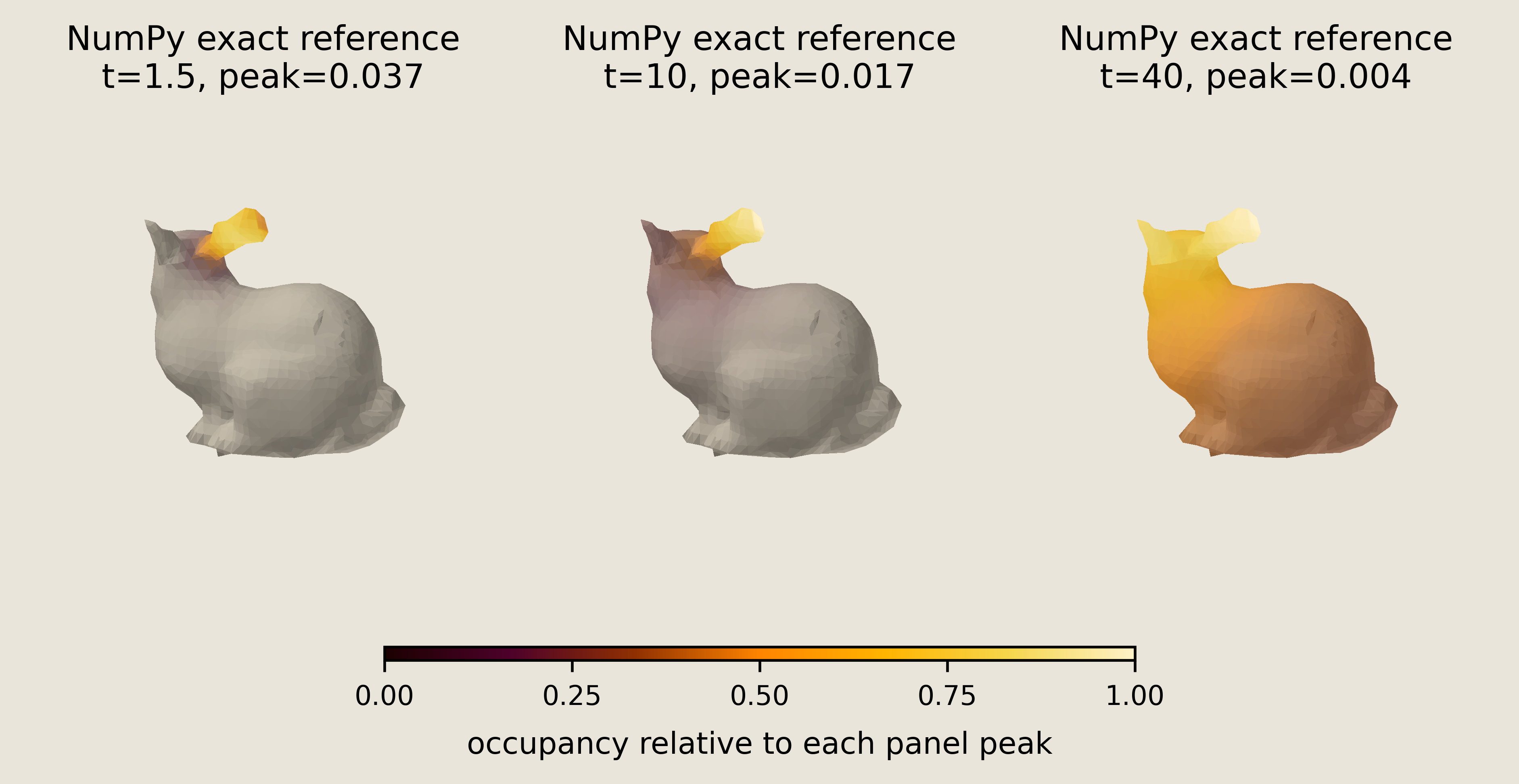
In the time sequence, the peaks reported in the titles fall from 0.037 at $t=1.5$ to 0.004 at $t=40$. By $t=40$, every vertex exceeds 15% of that panel's peak, and the field is only 0.0172 away in L2 from the uniform distribution. The final panel therefore represents near-uniform occupancy across the connected graph, not a localized front. Because each panel has its own normalization, the titles—not the colors across panels—show the decrease in absolute peak probability.
The same Torx primitive, checked on a patch
Each repetition of the full circuit applies 1,352 PSWAP gates, far too many to check by reading a picture of them, so we split the checking in two: we draw the primitive on a single edge, then run it on a graph small enough to compare vertex by vertex.
Every mesh edge contributes exactly one PSWAP, identical to notebook 02. The gate is structural, meaning the two-pbit circuit fixes the sites it acts on while one parameter fixes what it does with them: that parameter is the logit of $p$, identity occurs with probability $1-p$, and the states $10$ and $01$ swap with probability $p$.
example_pswap = DiscretePCircuit([PSWAP([0, 1])])
The schematic below encodes the two sites joined by a single gate and the parameter that sets their swap probability. It describes the local operation, but not the behavior of the repeated full-graph circuit.
fig = P_sch.draw_edge_pswap(example_pswap)
savefig(fig, "03_bunny_pswap_circuit")
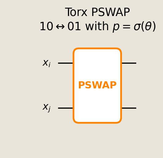
The full construction repeats this gate once per graph edge in each ordered layer, with the layer and repetition count shown above.
To check the repeated update directly, we compare Torx with the deterministic NumPy mean of the same ordered sweep on a 32-vertex patch grown outward from the source by breadth-first search (BFS).
We first close the patch by removing every edge from those 32 vertices to the rest of the bunny and retaining all edges among the 32 vertices. The resulting graph is the induced subgraph on the selected vertices. Closing it serves two purposes: probability cannot leave through a cut edge, and Torx and NumPy operate on exactly the same finite graph. This makes the comparison an implementation-parity check rather than an approximation of the full-graph field on a smaller domain. Removing the boundary edges changes the diffusion within the patch, so the patch result should not be interpreted as a cropped version of the full-graph result.
For this check, we use swap probability 0.12 for three repetitions. The code converts this probability to the equivalent unit-rate slice time and reports the patch's effective total time, which is distinct from the full-graph $t=1.5$ result.
PATCH_SIZE = 32
SWAP_PROBABILITY = 0.12
PATCH_REPS = 3
PATCH_SAMPLES = 4_000
PATCH_SEED = 17
PATCH_SLICE_TIME = -0.5 * np.log(1.0 - 2.0 * SWAP_PROBABILITY)
PATCH_EFFECTIVE_TIME = PATCH_REPS * PATCH_SLICE_TIME
# BFS from source to extract a connected patch.
adjacency = [[] for _ in range(len(vertices))]
for a, b in edges:
    adjacency[int(a)].append(int(b))
    adjacency[int(b)].append(int(a))
seen = {int(source)}
queue = deque([int(source)])
while queue and len(seen) < PATCH_SIZE:
    node = queue.popleft()
    for neighbor in sorted(adjacency[node]):
        if neighbor not in seen:
            seen.add(neighbor)
            queue.append(neighbor)
            if len(seen) >= PATCH_SIZE:
                break
patch_vertices = sorted(seen)
patch_index = {old: new for new, old in enumerate(patch_vertices)}
patch_edges = np.asarray(
    [
        (patch_index[int(a)], patch_index[int(b)])
        for a, b in edges
        if int(a) in patch_index and int(b) in patch_index
    ],
    dtype=np.int32,
)
ordered_patch_edges = tuple((int(a), int(b)) for a, b in patch_edges)
print(
    f"closed patch: {len(patch_vertices)} vertices, "
    f"{len(ordered_patch_edges)} internal edges, {PATCH_REPS} reps"
)
print(f"swap probability per edge: {SWAP_PROBABILITY}")
print(f"unit-rate effective time: {PATCH_EFFECTIVE_TIME:.3f}")
closed patch: 32 vertices, 84 internal edges, 3 reps
swap probability per edge: 0.12
unit-rate effective time: 0.412
We apply the same edge updates to probabilities instead of to sampled bits, which gives the ordered-sweep mean. Because it reuses the circuit's edge order, repetitions, and swap probability, any gap left between it and Torx is sampling error rather than a different update rule.
# The shared helper is also used for the deterministic full-graph mean above.
patch_initial = np.zeros(len(patch_vertices), dtype=float)
patch_initial[patch_index[int(source)]] = 1.0

deterministic_patch = ordered_pswap_product_formula_mean(
    patch_initial,
    ordered_patch_edges,
    reps=PATCH_REPS,
    swap_probability=SWAP_PROBABILITY,
)
Now the sampled side: the sample_pswap_product_formula helper builds the matching ordered Torx PSWAP circuit and estimates each vertex occupancy from one seeded batch of runs.
torx_patch = sample_pswap_product_formula(
    patch_initial,
    ordered_patch_edges,
    reps=PATCH_REPS,
    swap_probability=SWAP_PROBABILITY,
    num_samples=PATCH_SAMPLES,
    seed=PATCH_SEED,
)
patch_l2 = float(np.linalg.norm(torx_patch - deterministic_patch))

print(f"Torx vs NumPy ordered-sweep mean L2 error: {patch_l2:.4f}")
Torx vs NumPy ordered-sweep mean L2 error: 0.0159
np.testing.assert_allclose(torx_patch.sum(), 1.0, atol=5e-3)

source_local = patch_index[int(source)]
fig = P_samp.patch_parity_figure(
    deterministic_patch,
    torx_patch,
    source_index=source_local,
    l2_error=patch_l2,
    num_samples=PATCH_SAMPLES,
    seed=PATCH_SEED,
)
savefig(fig, "03_bunny_torx_patch_check")
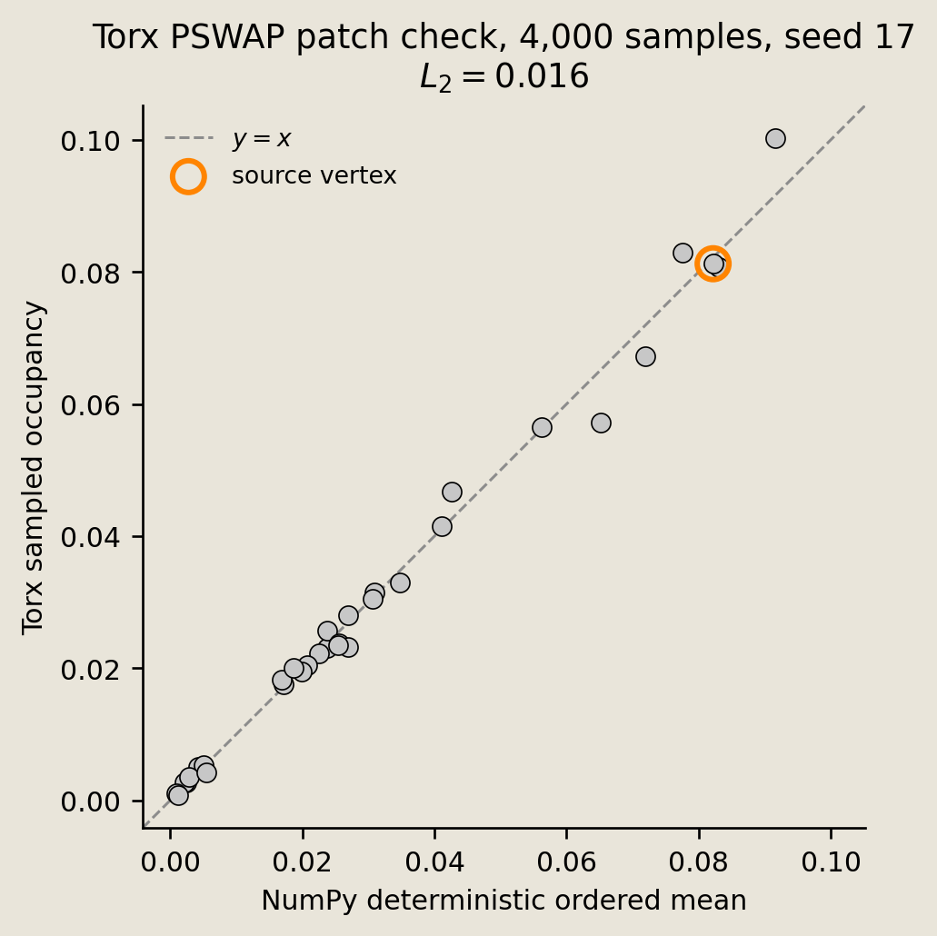
Across the 32 patch vertices, one seeded Torx run and the NumPy deterministic mean of the same closed-patch circuit differ by 0.0159 in L2, and the scatter shows where that difference sits vertex by vertex. The orange ring marks the source vertex.
Conclusion
We began with the bunny mesh, retained only its connectivity, and used one edge-local PSWAP factor for each term in the graph Laplacian. This construction produced three related fields whose comparisons distinguish sampled execution from the finite ordered approximation.
- The decimated mesh defines a 450-vertex, 1,352-edge graph from adjacency alone. It represents connectivity rather than mesh geometry and is not a geometry-aware model of physical heat.
- Torx applies one
PSWAPper edge for 11 repetitions and supplies the primary multi-seed sampled result at $t=1.5$. - NumPy supplies the deterministic ordered-sweep mean, the exact eigensolution, all error metrics, and the $t=10$ and $t=40$ references. Torx does not sample the later times because doing so would require many more repetitions of every gate.
- Comparing Torx with the ordered-sweep mean isolates sampling error; comparing that mean with the exact field isolates splitting bias; and comparing Torx directly with the exact field gives the total error.
- On the closed 32-vertex patch, a seeded Torx run and the matching NumPy ordered mean use the same finite graph and effective time, allowing their occupancies to be compared vertex by vertex.
See also:
- Notebook 02, the same construction on small graphs.
- Notebook 04, how
Branchingturns a circuit into samples.Simulator
References
- Trotter, H.F. 1959. On the product of semi-groups of operators. Proc. Amer. Math. Soc. 10(4), 545-551. The ordered per-edge product formula used here.
- Stanford Computer Graphics Laboratory. Stanford Bunny, zipper reconstruction, file
bun_zipper_res3.ply. Distributed through the Stanford 3D Scanning Repository, which requests source acknowledgment.